Protein Structure Determination

Contraints for Structure Calculation

So far, the emphasis has been on identification of the observed signals in the spectra and their correlation with the amino acid protons giving rise to the signals. Afterwards, one has to extract the data which are relevant for the structure. Of special importance in this respect are proton-proton distances, which can be estimated from the signal intensities in the 2D NOESY, 3D ¹⁵N-NOESY-HSQC and 3D ¹³C-NOESY-HSQC spectra .

Signal intensity depends on the distance r between two nuclei i and j, according to:

NOE_ij ~ 1/r_ij⁶

Distances are derived from the spectra after calibration against NOE signals for known distances (such as distances in elements of secondary structure) and grouped into a few classes. An upper and a lower bound of distance is assigned to each class. The lower bound is often set to the sum of the van der Waals radii of the two protons.

NOE class distance [Å] upper bound [Å]

very strong 2.3 2.5

strong 2.8 3.1

medium 3.1 3.4

weak 3.5 3.9

very weak 4.2 5.0

In this procedure, all non-sequential signals which are visible in the NOESY spectra have to be assigned, the number of which easily exceeds 1000 in a medium-sized protein (ca. 120 amino acids). It is distinguished between cross peaks of protons no more than five amino acids apart in the protein sequence (medium range NOE's) and those which are more than five amino acids apart (long range NOE's). The former are mainly indicative of the protein backbone conformation and are used for secondary structure determination, whereas the latter are an expression of the global structure of the protein and therefore contain the main information used for tertiary structure calculation.

In addition to interproton distances the phi-dihedral angles of the protein backbone can be determined from a COSY spectrum or a HNCA-J spectrum (a variant of the HNCA spectrum, from which the coupling constants of the N-C^alpha bonds can be determined). Dihedral angles are connected with the coupling constants via the Karplus equation .

Determination of Secondary Structure

I would have written a chapter about the determination of protein secondary structure by NMR spectroscopy by myself. But the offcial chapter "Determination of Protein Secondary Structure by NMR Spectroscopy" from Doc. Kurt D. Berndt of the Department of Medical Biochemistry and Biophysics, Karolinska Institute, which is found in section 8 of the PPS course material, is much better than my own version of the story would ever have been.

So may I invite you all to read his chapter about that topic and return to this page afterwards?

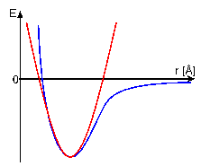
Calculation of Tertiary Structure

The idea of computer-aided structure calculation is to convert distance- and torsion-angle-data (constraints) into a visible structure. However, the experimentally determined distances and torsion angles by themselves are not sufficient to fully characterize a protein structure, as they are based on a limited number of proton-proton distances. Only the knowledge of empirical input data, such as bond lengths of all covalently attached atoms and bond angles, enables a reasonably exact structure determination.

For this purpose, a randomly folded starting structure is calculated from the empirical data and the known amino acid sequence. The computer program then tries to fold the starting structure in such a way, that the experimentally determined interproton distances are satisfied by the calculated structures. In order to achieve this, each known parameter is assigned an energy potential, which will give minimal energy if the calculated distance or angle coincides with its input value. The computer program tries to calculate a structure with a possibly small overall energy.

Without the experimentally determined distance- and torsion angle-constraints from the NMR spectra, the protein molecule can adopt a huge number of conformations due to the free rotation around its chemical bonds (except for the peptide bond, of course). the N-C^alpha bond and the C^alpha-CO bond. All these possible conformations are summed up in the so-called conformational space. Therefore, it is important to identify as many constraints as possible from the NMR spectra to restrict the conformational space as much as possible, thus getting close to the true structure of the protein. In fact, the number of constraints employed is more important than the accuracy of proton-proton distances, so that the classification above is sufficiently precise.

There are various computer programs, employing two in principle different methods for calculating a protein structure in solution:

Distance geometry (DG): This method is based on a calculation of matrices of distance constraints for each pair of atoms from all available distance constraints, bond and torsion angles as well as van der Waals radii. This set of distances is then projected from the n-dimensional distance space into the three-dimensional space of a cartesian coordinate system, in which it determines the coordinates of all atoms of the proteins.
Simulated Annealing (SA): This is a molecular dynamics method, which takes place directly in the cartesian coordinate system. In this method, a starting structure is heated to a high temperature in a simulation (i.e. the atoms of the starting structure get a high thermal mobility). During many discrete cooling steps the starting structure can evolve towards the energetically favourable final structure under the influence of a force field derived from the constraints.

The Simulated Annealing Method

As SA is much easier to understand than DG, we will concentrate on SA in the following text.

Energy Potentials

A starting structure is needed for a molecular dynamics calculation, which is generated from all constraints for the molecular structure, such as bond-lengths and bond-angles. This starting structure may be any conformation such as an extended strand or an already folded protein. During the simulation, it develops in a potential field under the influence of various forces, in which all information about the protein is summarized. Two classes of energy terms are distinguished: E_empirical and E_effective:

V = E_empirical + E_effective

with:

E_effective = E_NOE + E_torsion,

and

E_empirical = E_bond + E_angle + E_dihedral + E_vdw + E_electr

E_empirical contains all information about the primary structure of the protein and also data about topology and bonds in proteins in general. Structure family of severin The contributions of covalent bonds, bond-angles and dihedral angles towards E_empirical are approximated by a harmonic function. In contrast, non-covalent van-der-Waals forces and electrostatic interactions are simulated by an inharmonic Lennard-Jones potential or Coulomb potential, respectively. E_effective takes the experimentally determined constraints into account. Angle constraints are introduced by a harmonic function analogous to that for the dihedral angles. For distance constraints, the energy potential will be set to zero, if the corresponding distance is within the given limits. If it is outside these limits, a harmonic energy potential is used, which tries to push the value of the distance into the limits.

The SA Protocol

For a better understanding of the SA protocol have a look at this flow diagram of SA (13 k)

At the beginning of the calculation, the starting structure is energy minimized by moving the atoms of the starting structure, until it reaches an energy minimum. As a result of this process, a structure is obtained which is normally in a local minimum, without satisfying the constraints over vast regions. Such structures cannot reach the global energy minimum by further energy minimization, as they cannot cross the energy barrier between local and global minimum.

However, this energy barrier can be overcome if the necessary energy is put into the system. This is achieved by simulating the heating of the system up to a few thousand Kelvin via a coupled temperature bath. At this temperature the system receives enough energy to cross the energy barrier. Now, the system once again develops in energyhyperspace under the influence of the potential field.

The atomic positions at the end of a simulations step are determined from their starting positions, as well as from their velocities and accelerations, which in turn are both derived from the starting positions. Velocities can be calculated from the Maxwell distribution at a given temperature and accelerations are determined by Newton's equation from the force field. After a simulation step the energy potential is recalculated for the new atomic positions and a further simulation step follows. This procedure is iterated, searching the energyhyperspace for a global minimum.

After a previously chosen number of simulation steps at high temperature (up to 6000 times), atomic velocities (i.e. temperature) are slowly reduced in many steps (usually ca. 3000). At each temperature, the system is once again left to develop under the influence of the potential field. While the temperature of the system is reduced, simultaneously the force constants in the experimental constraints are raised in order to weigh them more strongly.

The result of the simulation is a minimum energy protein structure, but it cannot be excluded that this structure is stuck in a local minimum without ever reaching the global minimum, which is only marginally lower in energy. Therefore, about twenty different starting structures with random folds are used, which reach their final structure via different paths in energyhyperspace. These resulting structures are iteratively re-used as starting structures for another SA with slightly changed input protocolls, until no further reduction in global energy is observed and the structures converge in conformational space.

Results - The Structure Family

After the structural calculations a family of structures is obtained instead of an exactly defined structure. This family spans out a relatively narrow conformational space. Therefore, the quality of a NMR structure can be defined by the mean deviation of each structure from this family (RMSD) from an energy minimized mean structure which has to be calculated previously. The smaller the deviation from this mean structure the narrower the conformational space. Another definition of RMSD is to compare pairwise the structures of a family and calculate the mean of these deviations.

The RMSD is different for different parts of the protein structure: Regions with flexible structure or without secondary structure (loops) show a larger deviation than those with rigid and well defined secondary structure. This higher RMSD in loops results in first instance from the smaller number of distance constraints for these parts of the protein structure. Additionally it can originate from real flexibility, but this diagnosis can only be confirmed by measuring the relaxation times for the protein.

A result of a structure calculation is shown here:

This MOLSCRIPT-picture (suitable for stereo viewing) shows a ribbon plot of the averaged structure of the protein DS111M.

You can also view this structure with RasMol:

Here is the pdb file (126k) of the averaged structure of severin.

Try this rasmol script to viev the protein backbone colored according to secondary structure.

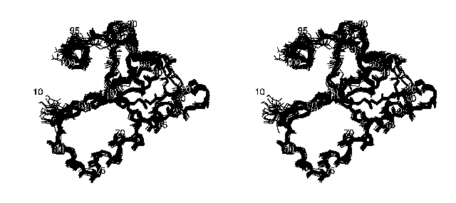
The following stereo picture shows the family of the 20 final structures of the protein DS111M:

Only the backbone atoms are shown in this picture for the sake of clarity. The orientation of the molecule is the same as in the picture above.

The accuracy in this family of structures can be displayed by another method: The following picture shows the backbone of DS111M as a cylindrical "sausage" of variable radius, which represents the global displacements among the 20 model structures in the structural family:

If you like to see it with rasmol here is a pdb file (2.3 MB!) with the family of 20 structures of severin.

Try this rasmol script to viev only the protein backbone of the structures colored with ramol standard colors according to secondary structure.

The calculation of this structure was performed with 1011 distance and 55 torsion angle constraints. This example illustrates the importance of a large number of constraints for obtaining a well defined NMR structure.

Horst Joachim Schirra's PPS2 project
Determination of Protein Structure with NMR Spectroscopy
last updated 281196

NOE class	distance [Å]	upper bound [Å]
very strong	2.3	2.5
strong	2.8	3.1
medium	3.1	3.4
weak	3.5	3.9
very weak	4.2	5.0